Gauss Labs
PEMF Device & Accessory Analysis
Report Status: Final

Purpose

This is the independent analysis of the MP7 paired with the MP7. The numbers come from direct measurements taken on calibrated lab instruments. What follows is what the pairing actually produces in a controlled environment, not what the data sheet claims.

Report Generated
October 5, 2026
Report ID
T2609191800
Test Engineer
David Dienhart
Test Date
October 3, 2026
Customer
Gauss Labs - A Division of Daboo Designs LLC
Device
MP7
Device #
D2609191710
Device Serial #
MP000054467
Accessory
MP7
Accessory #
A2609191735
Probe Orientation
Axial
App Version
4.0.369

Amendment: Amendment 2 of Report T2609191800. It supersedes the report finalized on 2026-09-20. Reason: Test using Fine resolution.

Device Notes: Modified Device

Accessory Notes: Modified Accessory

Executive Summary

The MP7 paired with the MP7 accessory was tested at each of its 2 settings, each producing a sawtooth wave. The four cards below show the most important metrics: slew rate, peak field strength, effective field diameter, and operating frequency. Secondary metrics and detail for each device setting follow in the rest of the report.
Slew Rate
Slew Rate
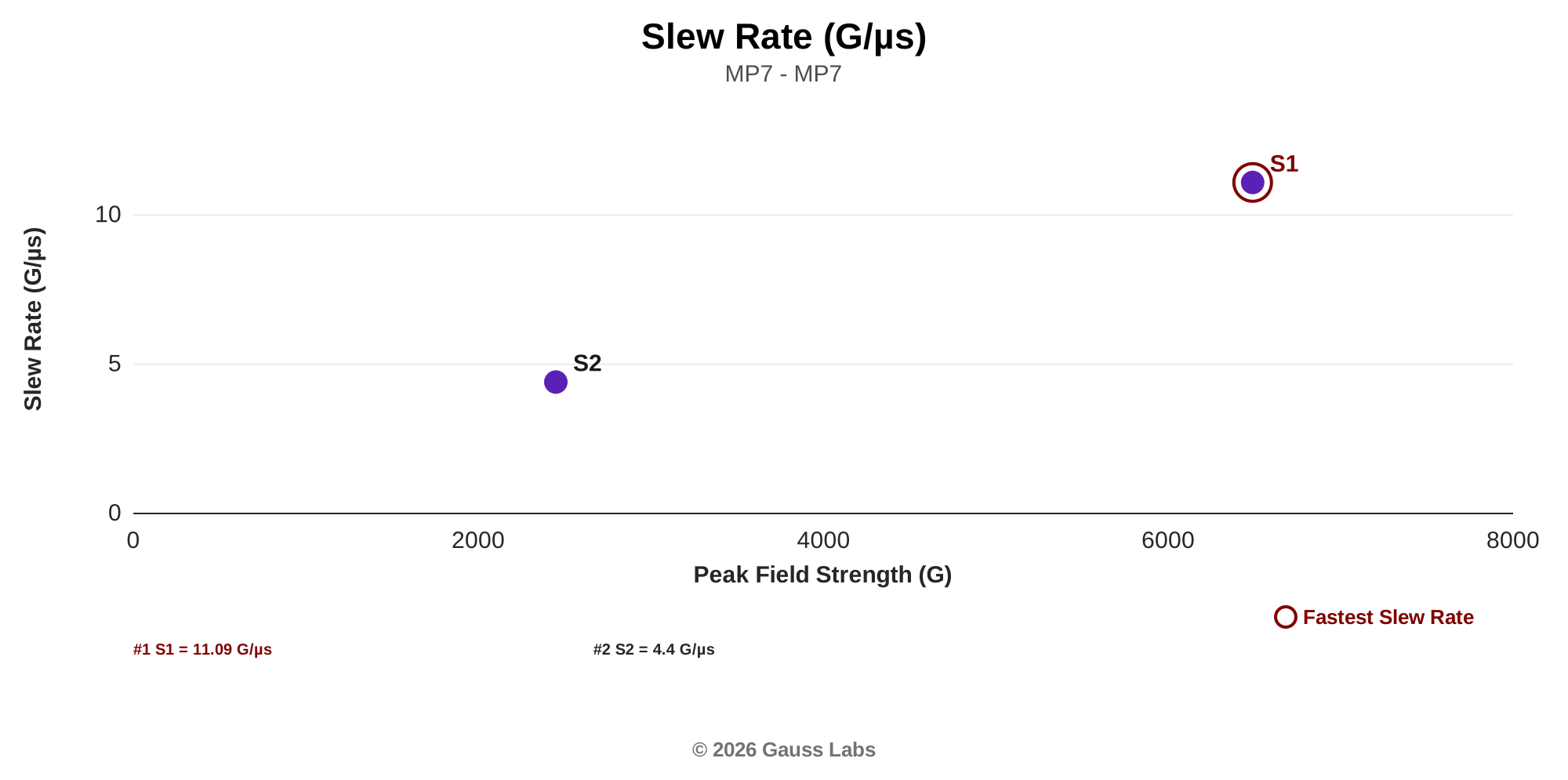
Slew rate is how fast the field changes during each pulse, measured in Gauss per microsecond (G/µs). Think of it like a hose: a sudden burst of water hits harder than a slow steady stream, even at the same pressure. What reaches tissue tracks how quickly the field changes, more than how strong it gets, so slew rate is the primary driver of the induced stimulus. It is also the property safety guidelines watch most closely. The ICNIRP guidelines set exposure limits based on how fast a field changes, since a fast enough change is what begins to stimulate nerves. Those limits are described in Tesla per second, where 1 G/µs equals 100 T/s. They come from medical imaging and workplace exposure, so they are a useful reference point here, not a pass-or-fail mark for a wellness device. Slew rate rises with field strength, so each setting's value is measured at that setting's peak field, and the report states that field alongside the number so the two are read together. The legend below lists every setting; #1 marks the fastest.
Peak Field Strength
Peak Field Strength
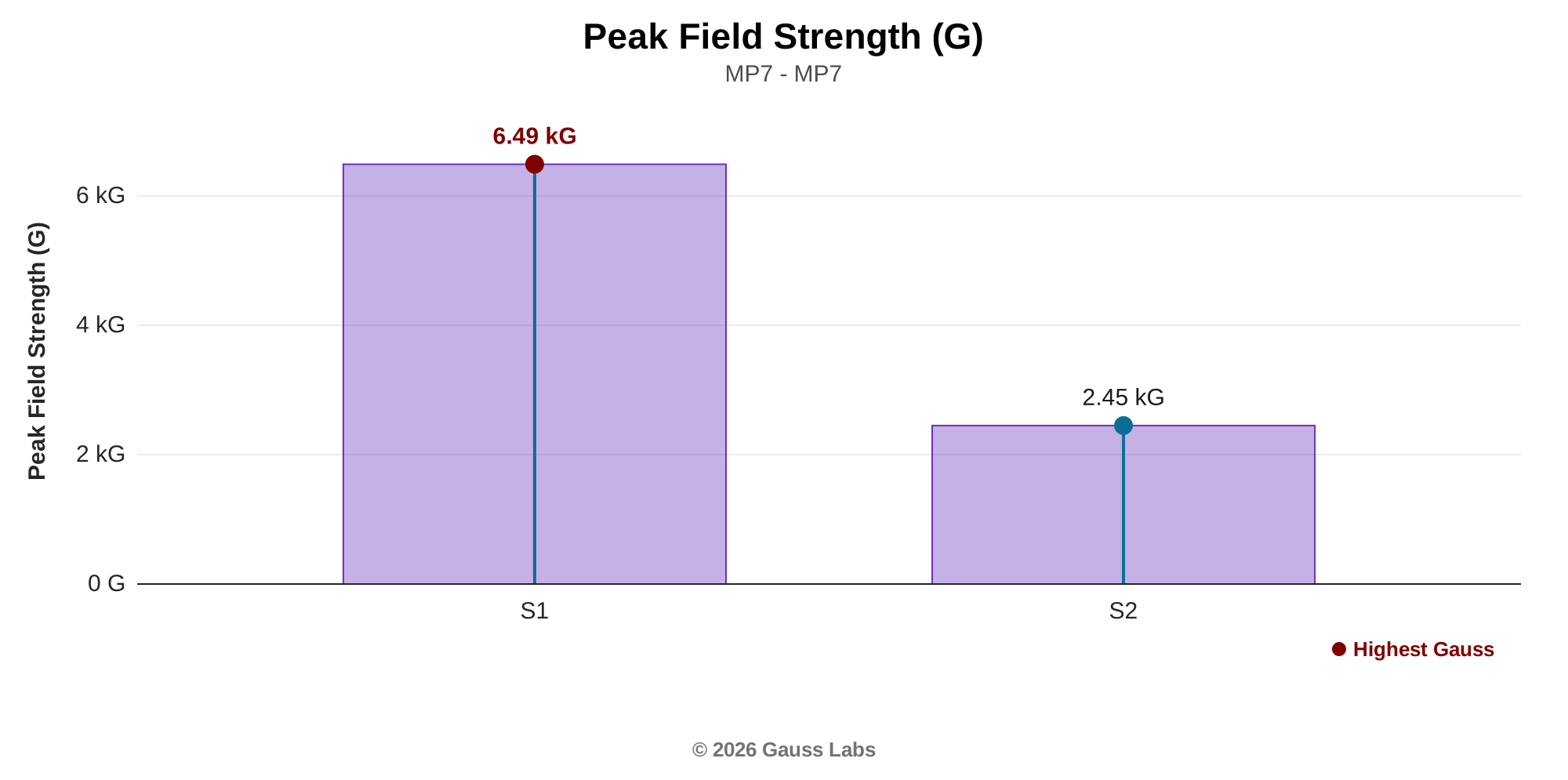
Peak field strength is how strong the magnetic field gets at its highest point, measured in Gauss (G). Think of it like the volume on a stereo: turning it up makes the music louder and the beat hits harder. Higher peaks carry more energy per pulse and keep the field above a usable level farther from the surface. At these low frequencies the body barely absorbs the field, so that reach carries into tissue rather than stopping at the surface. Each bar shows one setting; the tallest is the strongest.
Effective Field Diameter
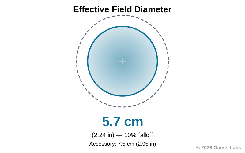
Effective Field Diameter is how wide the useful field is, the span where the field stays above 10% of its peak strength. It shows how much of the target area a single placement covers. The filled circle is the effective field; the dashed ring is the accessory housing, and the field often reaches past it, so a larger diameter means a wider working area from the same coil. The field also reaches 16.9 to 21.9 cm (6.7 to 8.6 in) from the surface before fading to the 5 Gauss edge, with any figure past the deepest measured plane modeled from the measurements; the Penetration Depth section maps this in full.
Operating Frequency
Operating Frequency
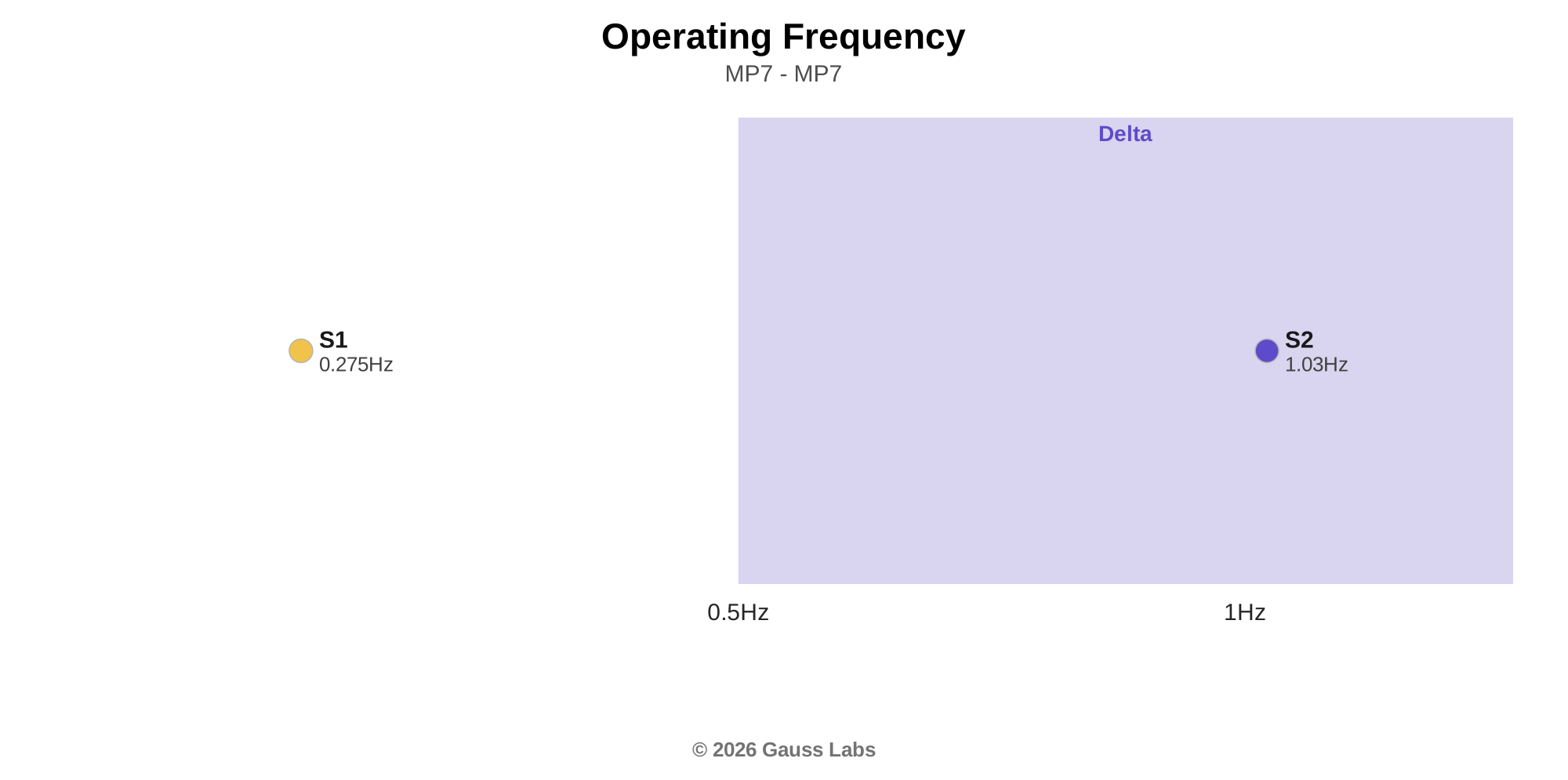
Operating frequency is how many pulses the device fires each second, measured in Hertz (Hz). The band names here (Delta, Theta, Alpha, Beta, Gamma) come from EEG naming and mark where each setting's frequency falls. They label the pulse rate, they do not promise a specific effect in the body. Each dot is one setting, placed in its band.

The MP7 paired with the MP7 was tested across multiple settings, using calibrated lab instruments instead of manufacturer-provided figures. The pairing matters: the same accessory on different devices, or different accessories on the same device, can produce measurably different results.

  • Slew rate, the speed at which the field changes during each pulse, peaks at 11.1 G/µs, measured where the field peaks at 6.49 kG. This is the measurement that most directly drives the induced stimulus in tissue.
  • Peak field strength ranges from 2.45 kG at the lowest setting to 6.49 kG at the highest. Gauss Labs groups this device in the higher-intensity range, which the lab sets at peaks above about 1,000 Gauss.
  • Total stimulation intensity, the cumulative biological effect delivered each second, peaks at 5.2 G/µs·Hz at the strongest setting. Higher values mean shorter sessions to achieve the same total effect.
  • Operating frequency spans 0.28 Hz to 1.03 Hz. A wide frequency range gives clinicians and users more settings to choose from on a single device.

Certification Readiness

This checklist shows how the MP7 paired with MP7 scored against each point of the Gauss Labs certification standard.

Functional pulse edge: Pass
The pulse has a real, functional rising edge, the basic requirement for any PEMF device.
Deliberate frequency: Pass
The device runs at a deliberate therapeutic frequency, clear of power-line interference.
Peak field strength: Pass
The accessory delivers a therapeutic field strength to the body.
Clean waveform: Pass
The device produces a clean, well-formed pulse.
Measured versus documented: Pass
The measured performance stays within tolerance of the documented specification.
Documented duty cycle: Not evaluated
This point was not evaluated; the test did not include the measurements it needs.
Documented pulse width: Not evaluated
This point was not evaluated; the test did not include the measurements it needs.
Field symmetry: Pass
The field reaches the body evenly in every direction around the accessory.

Field Coverage & Timing

The four cards below characterize the field shape and reach for the pairing as a whole. Together they describe how much total energy the accessory delivers, how concentrated the field is, how much cumulative stimulus each setting delivers, and how evenly the field distributes across the scan axes.
Total Effective Flux
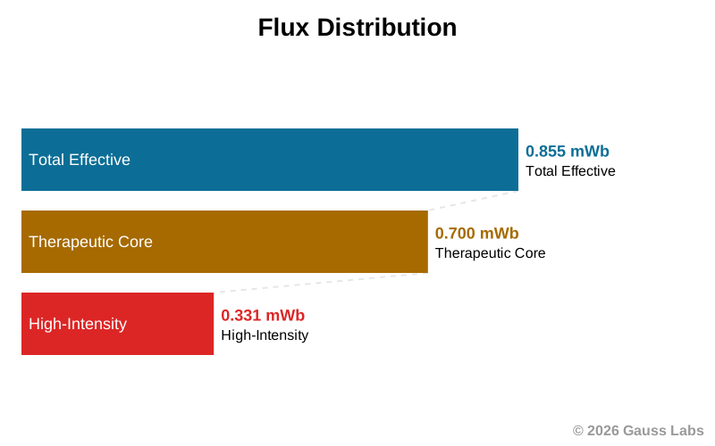
Total effective flux is the total magnetic energy delivered to the body during a single pulse, measured in milliweber (mWb). Think of water flow through a shower head versus a faucet: a shower fans the flow across a wide area; a faucet delivers it as a focused stream. Higher flux means stronger field, larger area, or both, which translates to greater coverage.
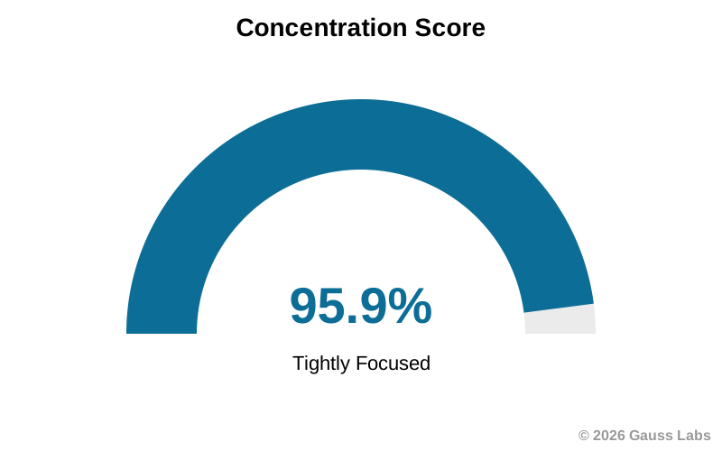
Concentration Score
Concentration Score
Concentration score is how tightly the field focuses on the target area, measured as a percentage of total field energy that lands inside the high-intensity zone. Think of it like a spotlight: a tight beam concentrates more energy in a small area; a wide beam spreads it out. Higher concentration delivers more energy to the target area; lower values give broader, gentler coverage.
Total Stimulation Intensity
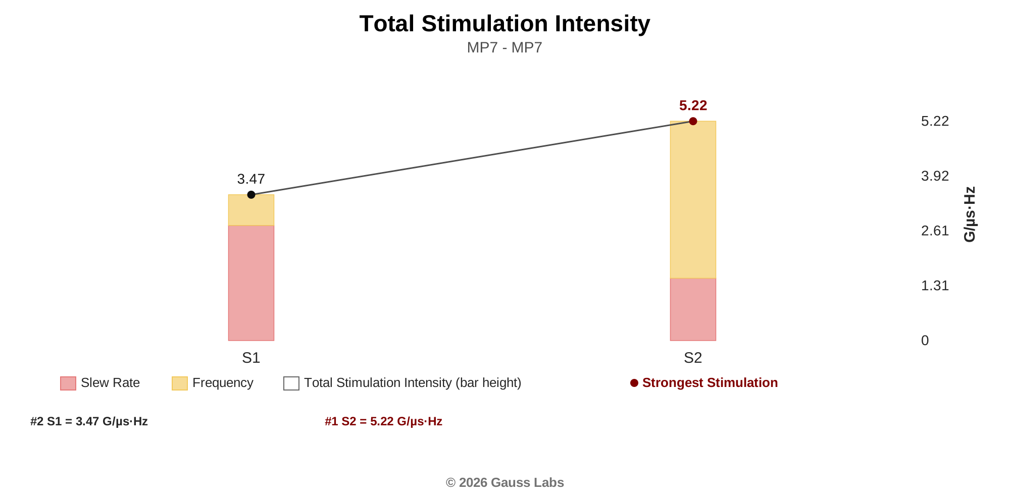
Total Stimulation Intensity combines two things into a single number: how fast the field changes (its slew rate) and how often it pulses (its frequency), measured in Gauss per microsecond per Hz (G/µs·Hz). Think of it like exercise, where harder effort done more often adds up to more total work. It captures the cumulative stimulus a setting delivers, so it favors settings that are both fast and frequent, not strong on just one. Each bar is one setting's combined result, and its two colors divide that height between the two ingredients, so a tall red section means the speed of the field is carrying the setting and a tall amber one means the pulse rate is.
Field Symmetry
Field Symmetry
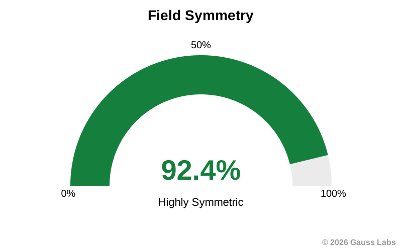
Field symmetry is how evenly the field reaches the body in every direction around the coil, measured as a percentage. Think of it like a balanced toy top: a balanced top spins smoothly on its axis; an unbalanced one wobbles. Higher symmetry means the field strength stays consistent in every direction; lower symmetry favors certain sides.

Together these four metrics describe the field the accessory produces at its surface. Each one measures a different property of that field: total energy, focus, cumulative stimulus, and evenness across the scan axes.

  • Total effective flux, the total magnetic energy delivered to the body per pulse, measures 0.855 mWb at the strongest setting. Higher flux means stronger field, larger area, or both.
  • Concentration score measures 95.9%. Higher concentration delivers more energy to the target area; lower values give broader, gentler coverage.
  • Total stimulation intensity measures 5.22 G/µs·Hz at the strongest setting. It combines how fast the field changes with how often it pulses, so it rewards settings that are both fast and frequent.
  • Field symmetry measures 92.4%. Higher symmetry means the field strength on every measured radial axis is nearly identical at every distance from center.

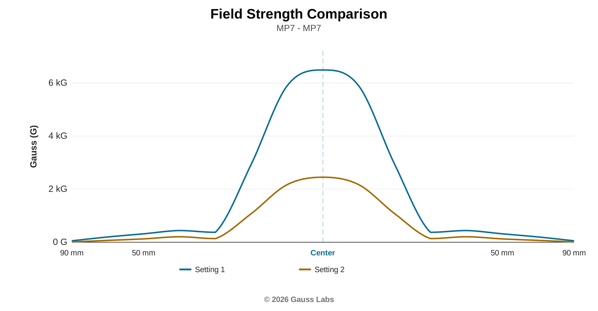
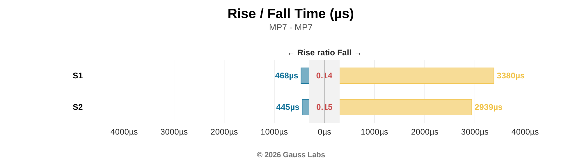
Field Strength Comparison overlays each setting's field strength as it falls off from the center of the accessory. Rise/Fall Time shows how long each pulse takes to turn on and how long it takes to turn off.

Field Strength Comparison
Field Strength Comparison

The Field Strength Comparison shows each setting's field strength from the center, horizontally measured moving outward. The chart's peaks represent the measurements taken from the points with the highest gauss readings.

Rise / Fall Time
Rise / Fall Time

Rise time is how quickly the field turns on. Fall time is how quickly it turns off. Both are measured in microseconds. Each pulse stimulates the body twice, once on the rise and once on the fall. How strongly each edge stimulates depends on its slew rate, the speed at which the field changes. A wide gap between rise and fall times means the rising and falling slew rates differ. The shorter edge has the higher slew rate.

Together these two views show the device's field strength and pulse timing for each setting tested.

  • Field Strength Comparison overlays each setting's field profile along the surface, with peaks from 2.45 kG to 6.49 kG. The plot shows the Gauss output measured horizontally outward along the accessory.
  • Rise / Fall Time shows rise times from 445.1 µs to 468.2 µs and fall times from 2939.1 µs to 3379.9 µs. How strongly each edge stimulates depends on its slew rate, the speed at which the field changes. A noticeable gap between rise and fall times means the rising and falling slew rates differ; the shorter edge has the higher slew rate.

Per-Setting Metrics

This section looks at each device setting on its own. Every setting gets its own charts and a table of measured values, the detail behind the summary metrics earlier in the report.

Setting 1

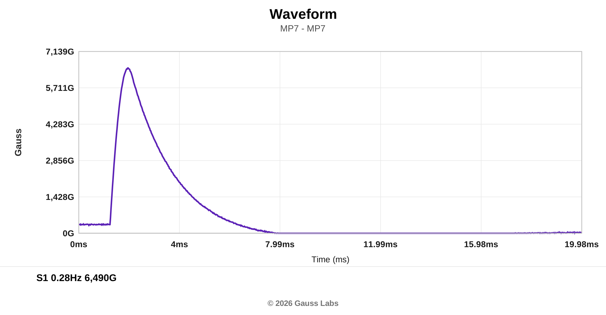
Waveform
Waveform

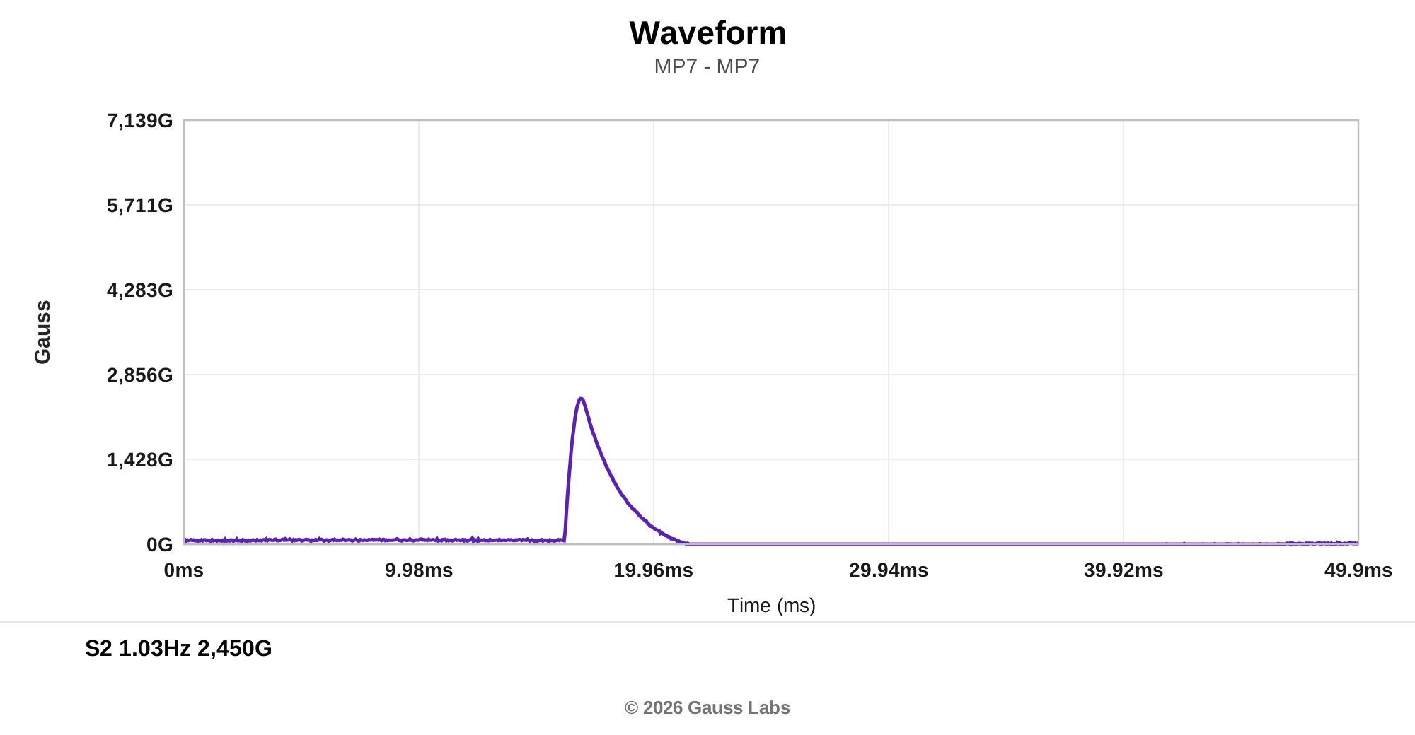
This pulse is a sawtooth wave: the field rises abruptly, then falls gradually. The fast edge does most of the work in the tissue.

Penetration Depth
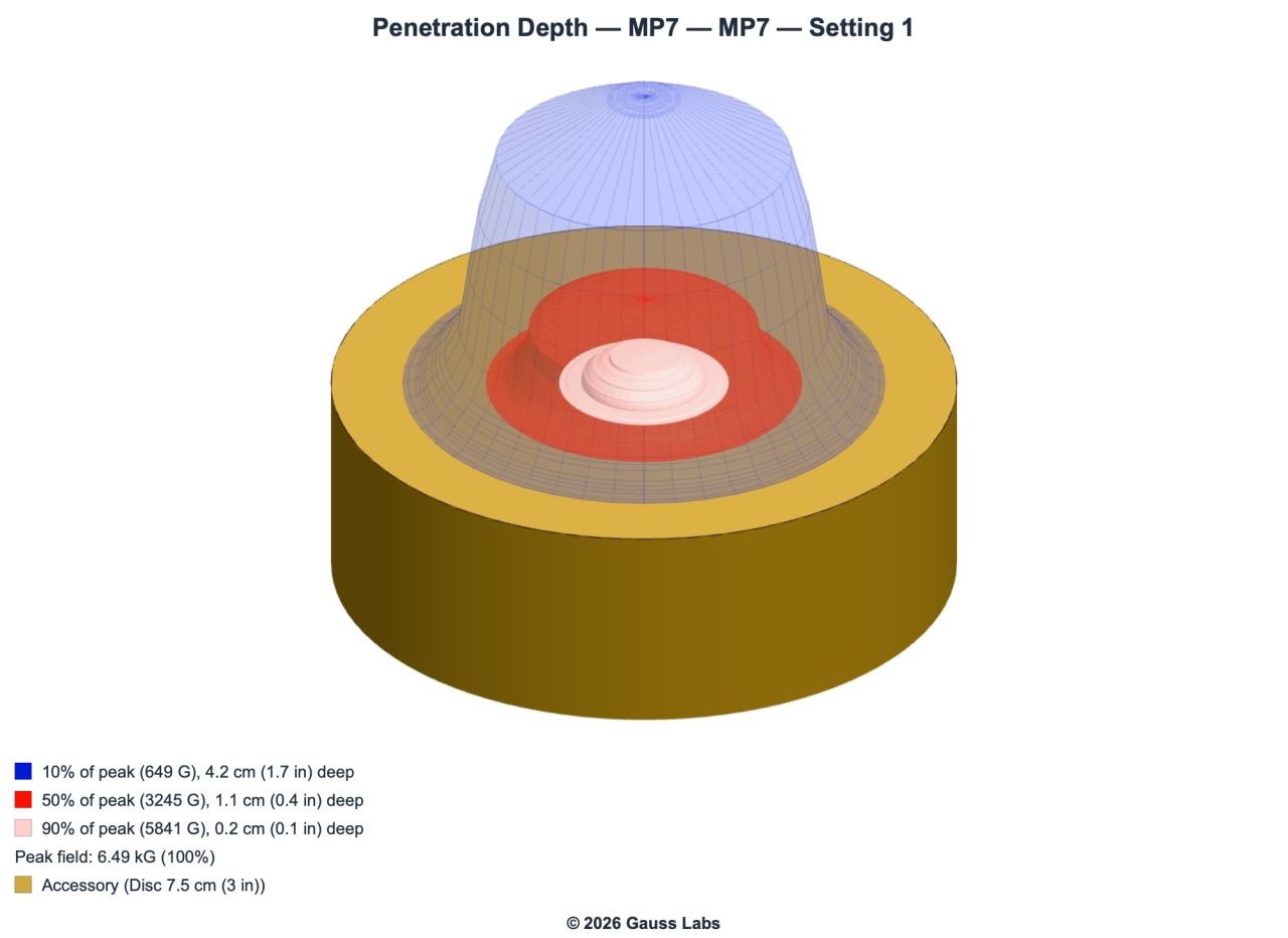
Penetration Depth

The chart shows the volume of space the field reaches above the accessory surface. The outer shell marks where the field drops to 10% of its peak, the practical edge of the field's reach. The inner shells mark 50% and 90% of peak, where the field is strongest near the accessory, and the legend gives each shell's depth. Distance is measured in open air above the accessory. At these low frequencies the body barely absorbs the field, so the same reach carries into tissue rather than stopping at the surface. Each setting's chart is framed to its own dome, so the legend depths are the way to compare settings.

Field Heatmap (surface)
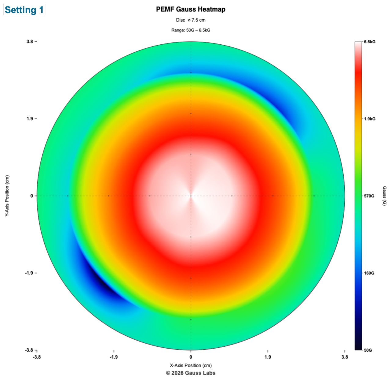
Field Heatmap (surface)

Top-down view of the field strength across the accessory surface. Warm colors represent higher Gauss; cool colors represent lower Gauss. The color scale spans this setting's own peak. A weaker setting therefore reads as clearly as the strongest.

Waveform at the CoilSawtooth (documented: Square)
Frequency0.28 Hz (doc: 0.3 Hz, -8.3%)
Peak Field Strength6.49 kG (doc: 7.00 kG, -7.3%)
Rise Time468.2 µs
Fall Time3.38 ms
Pulse Width1.767 ms
Duty Cycle0.05%
Slew Rate11.09 G/µs (1,109 T/s)
Total Stimulation Intensity3.47 G/µs·Hz
Penetration Depth (5 G edge)21.9 cm (8.6 in), modeled

Setting 2

Waveform

Waveform

This pulse is a sawtooth wave: the field rises abruptly, then falls gradually. The fast edge does most of the work in the tissue.

Penetration Depth
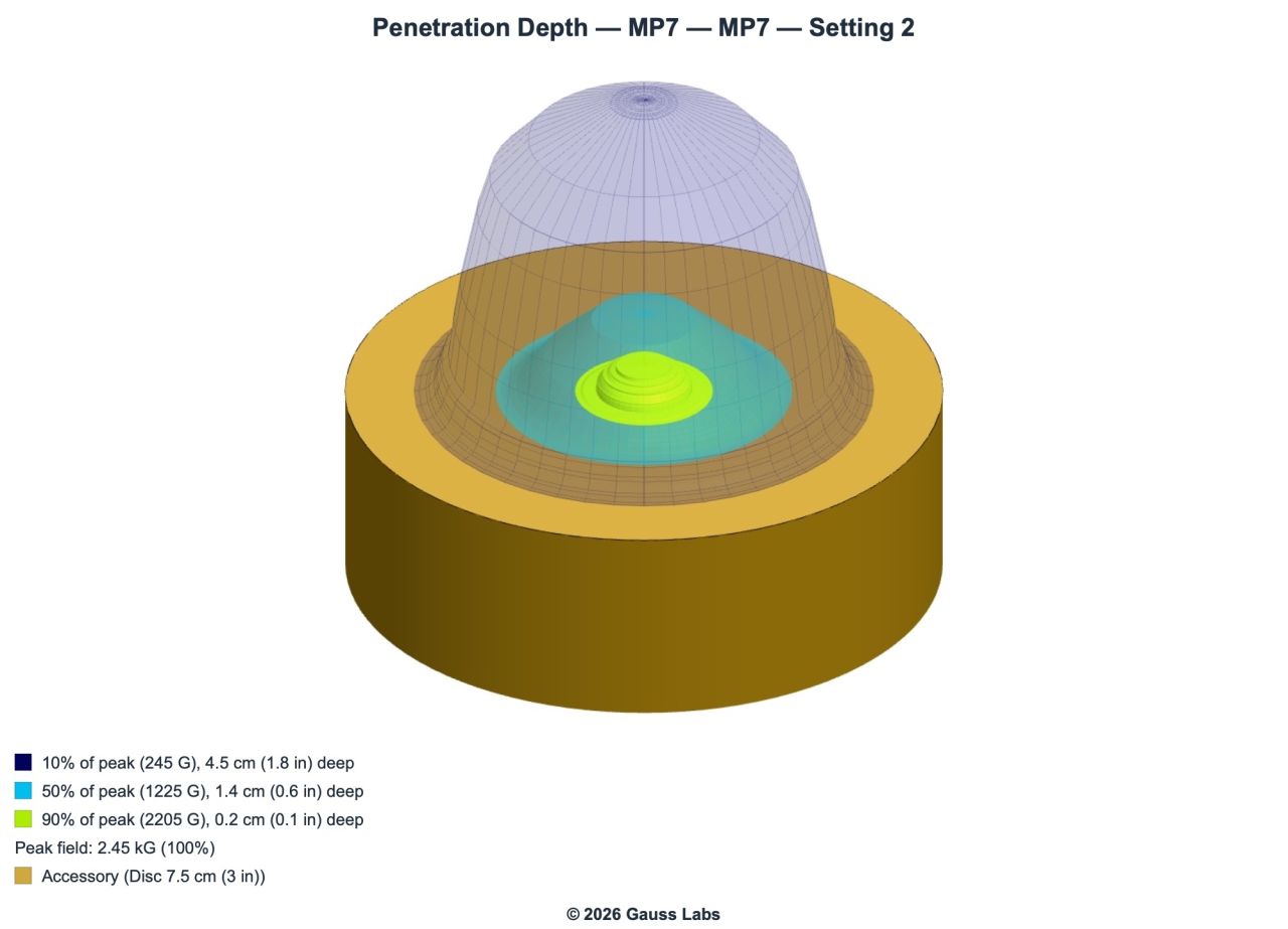
Penetration Depth

The chart shows the volume of space the field reaches above the accessory surface. The outer shell marks where the field drops to 10% of its peak, the practical edge of the field's reach. The inner shells mark 50% and 90% of peak, where the field is strongest near the accessory, and the legend gives each shell's depth. Distance is measured in open air above the accessory. At these low frequencies the body barely absorbs the field, so the same reach carries into tissue rather than stopping at the surface. Each setting's chart is framed to its own dome, so the legend depths are the way to compare settings.

Field Heatmap (surface)
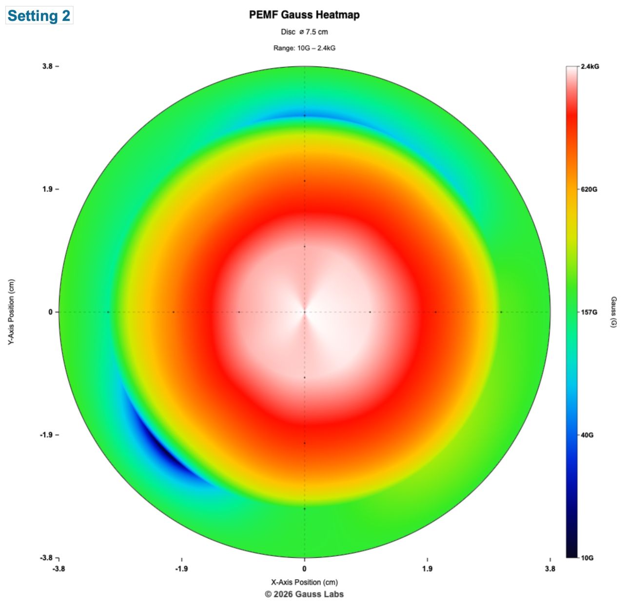
Field Heatmap (surface)

Top-down view of the field strength across the accessory surface. Warm colors represent higher Gauss; cool colors represent lower Gauss. The color scale spans this setting's own peak. A weaker setting therefore reads as clearly as the strongest.

Waveform at the CoilSawtooth (documented: Square)
Frequency1.03 Hz (doc: 1.1 Hz, -6.4%)
Peak Field Strength2.45 kG (doc: 3.50 kG, -30.0%)
Rise Time445.1 µs
Fall Time2.939 ms
Pulse Width1.674 ms
Duty Cycle0.17%
Slew Rate4.40 G/µs (440 T/s)
Total Stimulation Intensity5.22 G/µs·Hz
Penetration Depth (5 G edge)16.9 cm (6.7 in), modeled

Test Setup & Methodology

The test engineer measured each setting on calibrated laboratory instruments, recording the field strength, the waveform, and the supporting electrical readings. Conditions stayed consistent from one setting to the next, so the numbers compare cleanly across the report.

Scan Grid
Scan Grid

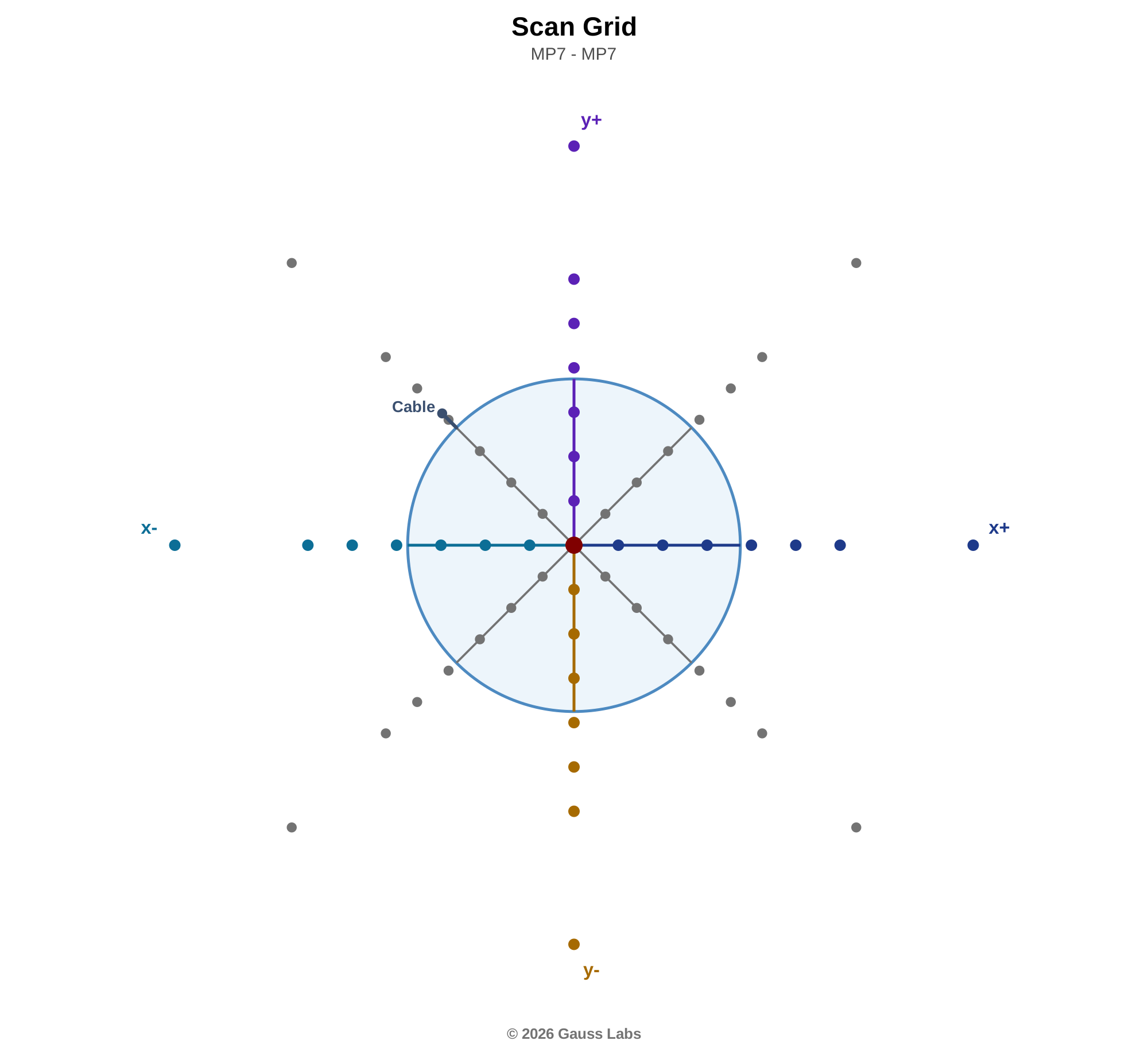
The diagram shows the accessory outline and the points along each axis where the test engineer placed the probe. The colored lines mark the four scan axes; the dots along each line are the probe positions.

Test Photos
Test photo 1

Test Setup

Device/Accessory Information

Analysis DateOctober 3, 2026
Device Under TestMP7
Operating Range0.3 Hz to 1.1 Hz
Applicator / AccessoryMP7
Settings Tested2 settings
Frequency Range0.28 Hz to 1.03 Hz
Waveforms at the CoilSawtooth Wave

Equipment

EquipmentMake and ModelTolerance
Gauss MeterAlphaLab Inc. MagWave (Serial 1012)Not stated
OscilloscopeRigol DHO814Not stated
Gauss MeterFW Bell 5180 (Serial FWB4)Low Range: 0.8% / 4 counts, Mid/High Range: 0.6% / 3 counts
Gauss Meter ProbeFW Bell Axial (Serial A1)Not stated
LCR MeterFNIRSI LC1020ENot stated
Field MapperGauss Labs Field MapperNot stated

Gauss Meter Probe: Gauss Meter Probe

LCR Meter: LCR Meter

Test Parameters

Accessory ShapeDisc (Round)
Measured AxesX-, X+, Y-, Y+, Z+
Scan Lines8
Points per Scan Line8
Total Scan Points513
Max Distance from Center9 cm (3.5 in)
Z-Axis Layers0 cm (Surface), 0.8 cm (0.3 in), 1.2 cm (0.5 in), 2.3 cm (0.9 in), 3.6 cm (1.4 in), 5.3 cm (2.1 in), 8.4 cm (3.3 in), 11.3 cm (4.4 in), 18 cm (7.1 in)
Z-Axis Layers, Setting 10 cm, 1.2 cm (0.5 in), 3.6 cm (1.4 in), 8.4 cm (3.3 in), 18 cm (7.1 in)
Z-Axis Layers, Setting 20 cm, 0.8 cm (0.3 in), 2.3 cm (0.9 in), 5.3 cm (2.1 in), 11.3 cm (4.4 in)
Point Spacing1 cm (0.4 in)
Measured OnGauss Labs Field Mapper
Ambient Field1.8 G (average of 3 readings with the device off)

Manufacturing Tolerance

A measured value won't always match the documented specification to the decimal, and that's expected. No two units come off a line exactly alike. Small differences in the parts, and in the wall power feeding the device, add up. In most cases they produce a 10% to 20% difference from that figure, and up to 30% in some. A reading in that range is normal.

The numbers in this report come from the specific unit and accessory the test engineer measured, under the conditions documented above. Another unit of the same model should land in a similar range, not with the exact same measurements.

Waveform Shape

The waveform named for each setting is the shape of the magnetic field measured at the coil. A manufacturer's specification usually names something different: the shape the device drives into the coil. The two rarely match, and both are right.

The field follows the current in the coil, and current cannot change instantly through a coil. So the coil rounds the edges of whatever it is given. A square drive arrives at the probe as a ramp or as a ring, which is why a device documented as a square wave is measured here as a sine or a sawtooth. The shape is reported for what it is, and a difference of this kind is not counted against the device.

Measurement Data

Per-setting measurement detail follows. Each setting is presented with the readings sheet data and the spatial scan grid grouped by z-plane.

Setting 1

Axes: rows below organize the four horizontal scan axes (x-, x+, y-, y+) plus the Center reading; depth planes follow as z-plane subsections beneath each axis block.

Frequency (Hz)0.28 Hz
Peak Field Strength6.49 kG
Documented Frequency (Hz)0.3 Hz
Documented Gauss (G)7,000

z = 0 cm

Distancex-axis - (G)x-axis + (G)y-axis - (G)y-axis + (G)
Center6.49 kG6.49 kG6.49 kG6.49 kG
1 cm (0.4 in)5.53 kG6.17 kG6.07 kG5.6 kG
2 cm (0.8 in)2.37 kG3.36 kG3.49 kG2.58 kG
3 cm (1.2 in)320 G540 G570 G210 G
4 cm (1.6 in)570 G320 G340 G540 G
5 cm (2 in)350 G280 G290 G350 G
6 cm (2.4 in)210 G180 G190 G210 G
9 cm (3.5 in)50.00 G50.00 G50.00 G50.00 G
Distance45° (G)135° (G)225° (G)315° (G)
1 cm (0.4 in)6.04 kG5.6 kG5.77 kG6.32 kG
2 cm (0.8 in)2.96 kG2.3 kG2.82 kG3.57 kG
3 cm (1.2 in)130 G380 G50.00 G780 G
4 cm (1.6 in)450 G540 G490 G270 G
5 cm (2 in)320 G340 G330 G270 G
6 cm (2.4 in)200 G210 G210 G180 G
9 cm (3.5 in)50.00 G60.00 G60.00 G50.00 G

z = 1.2 cm (0.5 in)

Distancex-axis - (G)x-axis + (G)y-axis - (G)y-axis + (G)
Center3.05 kG3.05 kG3.05 kG3.05 kG
1 cm (0.4 in)2.48 kG2.74 kG2.73 kG2.52 kG
2 cm (0.8 in)1.34 kG1.78 kG1.77 kG1.42 kG
3 cm (1.2 in)340 G740 G730 G410 G
4 cm (1.6 in)50.00 G150 G130 G10.00 G
5 cm (2 in)130 G20.00 G30.00 G110 G
6 cm (2.4 in)110 G60.00 G60.00 G100 G
9 cm (3.5 in)40.00 G30.00 G30.00 G40.00 G
Distance45° (G)135° (G)225° (G)315° (G)
1 cm (0.4 in)2.93 kG2.72 kG2.85 kG3.08 kG
2 cm (0.8 in)1.59 kG1.3 kG1.53 kG1.85 kG
3 cm (1.2 in)580 G320 G500 G820 G
4 cm (1.6 in)50.00 G60.00 G10.00 G190 G
5 cm (2 in)70.00 G130 G80.00 G0.00 G
6 cm (2.4 in)80.00 G110 G90.00 G50.00 G
9 cm (3.5 in)30.00 G40.00 G40.00 G30.00 G

z = 3.6 cm (1.4 in)

Distancex-axis - (G)x-axis + (G)y-axis - (G)y-axis + (G)
Center700 G700 G700 G700 G
1 cm (0.4 in)620 G670 G660 G620 G
2 cm (0.8 in)450 G540 G540 G460 G
3 cm (1.2 in)270 G370 G370 G290 G
4 cm (1.6 in)130 G220 G220 G140 G
5 cm (2 in)40.00 G110 G100 G50.00 G
6 cm (2.4 in)0.00 G40.00 G40.00 G0.00 G
9 cm (3.5 in)0.00 G0.00 G0.00 G0.00 G
Distance45° (G)135° (G)225° (G)315° (G)
1 cm (0.4 in)690 G653 G684 G725 G
2 cm (0.8 in)500 G440 G500 G550 G
3 cm (1.2 in)330 G270 G320 G390 G
4 cm (1.6 in)180 G120 G170 G230 G
5 cm (2 in)80.00 G40.00 G70.00 G120 G
6 cm (2.4 in)20.00 G0.00 G10.00 G50.00 G
9 cm (3.5 in)0.00 G0.00 G0.00 G0.00 G

z = 8.4 cm (3.3 in)

Distancex-axis - (G)x-axis + (G)y-axis - (G)y-axis + (G)
Center97.00 G97.00 G97.00 G97.00 G
1 cm (0.4 in)92.00 G95.00 G97.00 G91.00 G
2 cm (0.8 in)79.00 G88.00 G89.00 G79.00 G
3 cm (1.2 in)68.00 G80.00 G79.00 G69.00 G
4 cm (1.6 in)54.00 G62.00 G61.00 G52.00 G
5 cm (2 in)39.00 G51.00 G48.00 G39.00 G
6 cm (2.4 in)24.00 G36.00 G38.00 G24.00 G
9 cm (3.5 in)0.00 G8.00 G8.00 G0.00 G
Distance45° (G)135° (G)225° (G)315° (G)
1 cm (0.4 in)106 G105 G106 G108 G
2 cm (0.8 in)86.00 G79.00 G82.00 G90.00 G
3 cm (1.2 in)73.00 G64.00 G73.00 G80.00 G
4 cm (1.6 in)59.00 G51.00 G58.00 G67.00 G
5 cm (2 in)43.00 G33.00 G46.00 G51.00 G
6 cm (2.4 in)31.00 G25.00 G29.00 G38.00 G
9 cm (3.5 in)4.00 G0.00 G1.00 G12.00 G

z = 18 cm (7.1 in)

Distancex-axis - (G)x-axis + (G)y-axis - (G)y-axis + (G)
Center9.40 G9.40 G9.40 G9.40 G
1 cm (0.4 in)9.70 G9.10 G9.40 G11.50 G
2 cm (0.8 in)8.40 G9.30 G8.40 G8.90 G
3 cm (1.2 in)7.60 G7.70 G8.00 G7.60 G
4 cm (1.6 in)6.00 G7.50 G9.20 G6.80 G
5 cm (2 in)6.80 G7.40 G7.50 G6.80 G
6 cm (2.4 in)5.80 G5.30 G5.70 G4.80 G
9 cm (3.5 in)3.10 G4.40 G3.00 G3.60 G
Distance45° (G)135° (G)225° (G)315° (G)
1 cm (0.4 in)10.50 G8.70 G11.10 G8.50 G
2 cm (0.8 in)9.30 G7.10 G9.60 G10.00 G
3 cm (1.2 in)8.80 G7.10 G7.10 G9.40 G
4 cm (1.6 in)7.70 G6.70 G7.40 G8.90 G
5 cm (2 in)5.80 G5.10 G5.10 G7.50 G
6 cm (2.4 in)6.50 G3.70 G5.30 G5.90 G
9 cm (3.5 in)2.20 G1.70 G2.30 G3.40 G
z = 20.1 cm (7.9 in)
LinePositionGauss (G)
r101 cm (0.4 in)5.60 G
r102 cm (0.8 in)4.90 G
r103 cm (1.2 in)6.10 G
r104 cm (1.6 in)5.70 G
r141 cm (0.4 in)5.60 G
r142 cm (0.8 in)5.10 G
r143 cm (1.2 in)4.40 G
r144 cm (1.6 in)4.70 G
r145 cm (2 in)4.00 G
r21 cm (0.4 in)4.20 G
r22 cm (0.8 in)5.40 G
r23 cm (1.2 in)4.70 G
r24 cm (1.6 in)4.80 G
r61 cm (0.4 in)4.60 G
r62 cm (0.8 in)4.60 G
r63 cm (1.2 in)4.00 G
x+0 cm5.20 G
x+1 cm (0.4 in)5.70 G
x+2 cm (0.8 in)5.90 G
x+3 cm (1.2 in)5.80 G
x+4 cm (1.6 in)3.80 G
x+5 cm (2 in)3.20 G
x-1 cm (0.4 in)5.30 G
x-2 cm (0.8 in)3.80 G
x-3 cm (1.2 in)4.50 G
x-5 cm (2 in)5.50 G
y+1 cm (0.4 in)3.00 G
y+2 cm (0.8 in)5.40 G
y+3 cm (1.2 in)5.50 G
y+4 cm (1.6 in)4.60 G
y+5 cm (2 in)3.70 G
y-1 cm (0.4 in)5.40 G
y-2 cm (0.8 in)4.50 G
y-3 cm (1.2 in)5.80 G
y-4 cm (1.6 in)4.60 G
y-5 cm (2 in)2.80 G

The readings at z = 20.1 cm (7.9 in) were taken above the deepest plane, only at the 36 strongest places, where the field was still above the climb target at z = 18 cm (7.1 in).

Setting 2

Axes: rows below organize the four horizontal scan axes (x-, x+, y-, y+) plus the Center reading; depth planes follow as z-plane subsections beneath each axis block.

Frequency (Hz)1.03 Hz
Peak Field Strength2.45 kG
Documented Frequency (Hz)1.1 Hz
Documented Gauss (G)3,500

z = 0 cm

Distancex-axis - (G)x-axis + (G)y-axis - (G)y-axis + (G)
Center2.45 kG2.45 kG2.45 kG2.45 kG
1 cm (0.4 in)2 kG2.28 kG2.21 kG2.08 kG
2 cm (0.8 in)810 G1.29 kG1.23 kG980 G
3 cm (1.2 in)120 G230 G180 G50.00 G
4 cm (1.6 in)250 G170 G190 G240 G
5 cm (2 in)130 G120 G120 G130 G
6 cm (2.4 in)70.00 G70.00 G70.00 G70.00 G
9 cm (3.5 in)10.00 G10.00 G10.00 G10.00 G
Distance45° (G)135° (G)225° (G)315° (G)
1 cm (0.4 in)2.23 kG2.07 kG2.12 kG2.34 kG
2 cm (0.8 in)1.15 kG830 G980 G1.33 kG
3 cm (1.2 in)80.00 G130 G10.00 G290 G
4 cm (1.6 in)220 G190 G230 G160 G
5 cm (2 in)130 G120 G130 G120 G
6 cm (2.4 in)70.00 G70.00 G70.00 G60.00 G
9 cm (3.5 in)10.00 G10.00 G10.00 G10.00 G

z = 0.8 cm (0.3 in)

Distancex-axis - (G)x-axis + (G)y-axis - (G)y-axis + (G)
Center1.65 kG1.65 kG1.65 kG1.65 kG
1 cm (0.4 in)1.35 kG1.51 kG1.48 kG1.39 kG
2 cm (0.8 in)636 G909 G889 G720 G
3 cm (1.2 in)43.00 G290 G259 G106 G
4 cm (1.6 in)87.00 G0.00 G0.00 G70.00 G
5 cm (2 in)80.00 G40.00 G48.00 G75.00 G
6 cm (2.4 in)56.00 G41.00 G43.00 G54.00 G
9 cm (3.5 in)15.00 G11.00 G13.00 G12.00 G
Distance45° (G)135° (G)225° (G)315° (G)
1 cm (0.4 in)1.25 kG1.16 kG1.22 kG1.31 kG
2 cm (0.8 in)823 G634 G733 G946 G
3 cm (1.2 in)207 G40.00 G131 G320 G
4 cm (1.6 in)30.00 G92.00 G51.00 G8.00 G
5 cm (2 in)60.00 G80.00 G67.00 G38.00 G
6 cm (2.4 in)47.00 G56.00 G49.00 G37.00 G
9 cm (3.5 in)15.00 G12.00 G11.00 G9.00 G

z = 2.3 cm (0.9 in)

Distancex-axis - (G)x-axis + (G)y-axis - (G)y-axis + (G)
Center589 G589 G589 G589 G
1 cm (0.4 in)491 G544 G537 G503 G
2 cm (0.8 in)306 G392 G385 G326 G
3 cm (1.2 in)133 G217 G208 G148 G
4 cm (1.6 in)25.00 G87.00 G83.00 G36.00 G
5 cm (2 in)0.00 G18.00 G14.00 G0.00 G
6 cm (2.4 in)10.00 G0.00 G0.00 G5.00 G
9 cm (3.5 in)4.00 G0.00 G3.00 G5.00 G
Distance45° (G)135° (G)225° (G)315° (G)
1 cm (0.4 in)466 G435 G456 G487 G
2 cm (0.8 in)358 G302 G339 G404 G
3 cm (1.2 in)182 G127 G165 G228 G
4 cm (1.6 in)61.00 G19.00 G51.00 G98.00 G
5 cm (2 in)4.00 G0.00 G0.00 G22.00 G
6 cm (2.4 in)1.00 G10.00 G1.00 G0.00 G
9 cm (3.5 in)1.00 G6.00 G2.00 G0.00 G

z = 5.3 cm (2.1 in)

Distancex-axis - (G)x-axis + (G)y-axis - (G)y-axis + (G)
Center116 G116 G116 G116 G
1 cm (0.4 in)104 G113 G112 G104 G
2 cm (0.8 in)86.00 G98.00 G94.00 G85.00 G
3 cm (1.2 in)60.00 G72.00 G74.00 G59.00 G
4 cm (1.6 in)34.00 G51.00 G50.00 G34.00 G
5 cm (2 in)16.00 G31.00 G28.00 G18.00 G
6 cm (2.4 in)1.00 G17.00 G13.00 G7.00 G
9 cm (3.5 in)0.00 G0.00 G0.00 G0.00 G
Distance45° (G)135° (G)225° (G)315° (G)
1 cm (0.4 in)108 G102 G105 G109 G
2 cm (0.8 in)90.00 G84.00 G93.00 G99.00 G
3 cm (1.2 in)67.00 G55.00 G65.00 G76.00 G
4 cm (1.6 in)46.00 G34.00 G39.00 G52.00 G
5 cm (2 in)25.00 G13.00 G22.00 G29.00 G
6 cm (2.4 in)7.00 G1.00 G7.00 G15.00 G
9 cm (3.5 in)0.00 G0.00 G0.00 G0.00 G

z = 11.3 cm (4.4 in)

Distancex-axis - (G)x-axis + (G)y-axis - (G)y-axis + (G)
Center13.20 G13.20 G13.20 G13.20 G
1 cm (0.4 in)13.90 G13.00 G17.10 G15.60 G
2 cm (0.8 in)13.40 G15.20 G12.50 G11.70 G
3 cm (1.2 in)9.90 G13.10 G14.50 G11.50 G
4 cm (1.6 in)8.10 G10.40 G10.30 G7.80 G
5 cm (2 in)6.40 G8.50 G9.90 G8.60 G
6 cm (2.4 in)3.50 G6.50 G9.10 G5.00 G
9 cm (3.5 in)0.40 G3.70 G3.90 G1.80 G
Distance45° (G)135° (G)225° (G)315° (G)
1 cm (0.4 in)12.70 G11.70 G13.90 G14.00 G
2 cm (0.8 in)12.40 G12.40 G13.40 G13.30 G
3 cm (1.2 in)11.70 G10.00 G10.50 G11.20 G
4 cm (1.6 in)12.40 G8.90 G8.00 G10.50 G
5 cm (2 in)7.80 G6.10 G10.20 G8.80 G
6 cm (2.4 in)6.10 G3.20 G5.20 G5.40 G
9 cm (3.5 in)2.20 G2.20 G2.20 G2.40 G
z = 13.4 cm (5.3 in)
LinePositionGauss (G)
r101 cm (0.4 in)6.70 G
r102 cm (0.8 in)7.00 G
r103 cm (1.2 in)5.00 G
r104 cm (1.6 in)6.00 G
r105 cm (2 in)4.30 G
r141 cm (0.4 in)8.60 G
r142 cm (0.8 in)7.50 G
r143 cm (1.2 in)6.40 G
r144 cm (1.6 in)4.80 G
r145 cm (2 in)4.30 G
r21 cm (0.4 in)7.30 G
r22 cm (0.8 in)7.40 G
r23 cm (1.2 in)5.30 G
r24 cm (1.6 in)7.20 G
r25 cm (2 in)3.30 G
r61 cm (0.4 in)5.90 G
r62 cm (0.8 in)6.40 G
r63 cm (1.2 in)5.50 G
r64 cm (1.6 in)4.70 G
x+0 cm8.20 G
x+1 cm (0.4 in)7.50 G
x+2 cm (0.8 in)7.10 G
x+3 cm (1.2 in)5.40 G
x+4 cm (1.6 in)4.30 G
x+5 cm (2 in)4.50 G
x-1 cm (0.4 in)8.70 G
x-2 cm (0.8 in)7.50 G
x-3 cm (1.2 in)5.80 G
x-4 cm (1.6 in)6.40 G
y+1 cm (0.4 in)6.80 G
y+2 cm (0.8 in)6.70 G
y+3 cm (1.2 in)5.70 G
y+4 cm (1.6 in)7.20 G
y+5 cm (2 in)5.80 G
y-1 cm (0.4 in)7.60 G
y-2 cm (0.8 in)6.60 G
y-3 cm (1.2 in)5.30 G
y-4 cm (1.6 in)6.10 G
y-5 cm (2 in)4.10 G
y-6 cm (2.4 in)3.50 G

The readings at z = 13.4 cm (5.3 in) were taken above the deepest plane, only at the 40 strongest places, where the field was still above the climb target at z = 11.3 cm (4.4 in).

References

Primary sources behind the measurements and methods in this report.

The full measurement methods and references, including the physics and measurement conventions behind these results, are published at https://gausslabs.tech/references/.

Key Terms

Defined terms used elsewhere in this report.

5 Gauss
5 Gauss is the field level the report uses as the edge of a device's useful reach. Where the report describes how far a field reaches, it measures out to the distance at which the field falls to 5 Gauss. This is a measurement reference, not a biological threshold. It was chosen so a reported reach reflects field that stands clearly above the background, and the report does not claim the field stops mattering below it. For context, the earth's natural magnetic field at the surface is about 0.3 to 0.5 Gauss, so 5 Gauss is roughly ten times the ambient background.
50% Falloff Distance
The distance from center where the average field strength drops to 50% of its peak value. A shorter 50% falloff distance indicates a more tightly focused field. A longer distance indicates broader coverage. This is a distance, not a zone boundary: the Therapeutic Core is defined at 35% of peak and extends further out than this.
Accessory
The applicator component that delivers the electromagnetic field to the body. Some manufacturers call it an attachment. It contains one or more coils or loops, wound conductors that generate a pulsed magnetic field when driven by the control unit. Accessories come in various form factors including pads, rings, wraps, and wands. Each is designed for different anatomical targets. The coil geometry inside the accessory (pancake, donut, loop, stacked) determines the shape, depth, and distribution of the resulting magnetic field.
Accessory Shape
The overall physical form of the applicator that delivers the field, such as a disc, a loop or ring, or a flat mat. Accessory shape sets how the field is laid out over the target area: a disc concentrates it in a small spot, a loop surrounds a limb, and a mat spreads it across a wide surface. The shape also determines how the field is measured and which coverage figures appear in the report.
Accessory Thickness
The physical thickness of the accessory housing in centimeters. It's used to position the probe at a consistent height above the device. For disc accessories, this is the depth from the top surface to the bottom. For loop accessories, it's the cross-section diameter of the tubing that encloses the coil. The thickness sets where the measurement surface sits and anchors the height axis of the 3D Field Volume chart and the standoff convention. Disc reports use the full thickness as the probe offset because the probe rests on the disc top. Loop reports use half the thickness because the probe sits at the tube centerline inside the tubing.
Ambient Field
The magnetic field already present where an accessory is tested, with the PEMF device switched off. It comes from the Earth's field and from electrical equipment nearby, and it can shift a little as the room changes over a long test. Gauss Labs reads the ambient field at the start of every test and again at the end, with the device off and the probe where the accessory sits. Those two readings let the analysis account for the room's own field, so the measurements reported for the device are more accurate. The report gives both readings in gauss. See Gauss Meter.
Bipolar Pulse
A pulse that reverses field direction partway through its cycle, so it induces current twice, on the swing out and on the swing back. A pulse that stays in one direction is monophasic (unipolar); one that reverses is biphasic (bipolar). The two swings are the two phases of one pulse, not two pulses, which is what makes the pulse count ambiguous unless it is stated; see Pulses Per Second (pps), and see Phase.
Coil Count
The number of individual coils inside a multi-coil accessory such as a mat or pad. Knowing the count tells you how the device distributes its field across the target area: a 4-coil mat covers a wider zone but each coil contributes a smaller share of the total drive than a single-coil disc would. Each coil's peak location is identified from the field measurements and reported individually, so you can compare output and positioning across all coils in the accessory.
Coil Inductance (L)
The coil's resistance to changes in current flow. It directly determines how fast the magnetic field can rise when power is applied. Higher inductance means slower field buildup but potentially stronger peak field. Measured in Henries (H) or millihenries (mH). Inductance increases with more turns and with ferrite or iron core materials. Combined with resistance, it sets the L/R time constant.
Coil Layout
The arrangement of coils inside a multi-coil mat: where each coil sits and how large it is. It shows which parts of the mat carry the field. The scan grid is planned around it, so the closest readings fall over each coil. When the coils have been mapped with Coil Discovery, the layout comes from that mapping. Otherwise it's read from where each coil's field peaks in the scan. Each coil's position is given as an offset from the mat's center, and an evenly spaced layout is described as a grid (for example, 3x2 at 100 mm pitch). When the manufacturer supplies a layout, it's recorded as the documented layout and compared with the measured one.
Coil Resistance (R)
The electrical resistance of the coil wire. It determines how much heat the coil produces during operation and how much voltage the device needs to reach peak current. Lower resistance means less wasted heat and more efficient energy delivery to the magnetic field. Measured in Ohms (Ω). Resistance decreases with thicker wire (lower AWG number) and increases with temperature.
Coil Shape
The winding pattern of a coil, most often a flat pancake spiral or a ring-shaped loop. From its measured field a coil is also classified as pancake (center-strong), donut (ring-strong), or loop.
Coil Type
A classification of the electromagnetic coil inside the accessory based on its measured field distribution. A Pancake Coil produces a center-dominant field with peak strength at the center and rapid falloff outward. A Donut Coil produces a ring-dominant field with peak strength in a ring around the center and a weaker center. A Loop Coil concentrates energy along the wire path. Coil type is detected automatically from the scan data by comparing ring zone field strength to center field strength. For multi-coil mats (rect shape), single-coil-type detection doesn't apply. Instead the report uses Coil Count, Coil Layout, and Coverage Uniformity to describe the mat's collective behavior.
Concentration Score
A percentage measuring how much of the total measured field intensity at the accessory surface lands in the therapeutic core (scan points where Gauss is at or above 35% of peak). It's calculated as the sum of Gauss values at those points divided by the total sum of all measured Gauss values within the coil boundary. This is a surface concentration metric. It measures lateral field distribution across the face of the accessory, not depth penetration. The threshold was 50% of peak before August 2026; it was lowered to 35% because 50% proved too strict a definition of a strong field, and scores published before that date are not directly comparable to scores published after it. Across the accessories Gauss Labs has measured at the current threshold, discs score between 74% and 98%, and loops and rings between 58% and 100%. The formula is geometry-independent, so the same calculation applies to all coil types. Compare scores within the same coil type for meaningful benchmarks.
Coverage Area
The portion of a multi-coil mat surface where the magnetic field exceeds a defined fraction of the peak. Reported in cm² and as a percentage of total mat surface at two thresholds: 35% of peak, which is the figure the report quotes and the same threshold the Concentration Score uses, and 10% of peak, the practical edge of useful field. Coverage tells you how much of the mat actually delivers meaningful intensity rather than fading between coils. The quoted threshold was 50% of peak before August 2026, so coverage figures published before that date read lower than figures published after it for the same mat.
Coverage Uniformity
How consistent the per-coil peak field is across a multi-coil mat. Reported as the coefficient of variation (CV = standard deviation divided by mean) of detected coil peaks, expressed as a percent. Lower CV means tighter coil-to-coil consistency. Under 5% is tight uniformity (well-matched coils, consistent drive). 5–15% is moderate. Over 15% is a wide spread that may indicate construction variance or measurement positioning issues. The metric excludes the surface (z=0) center field and uses each coil's local peak as the comparison anchor.
Cross-Section
A view of the magnetic field as if the accessory were sliced vertically down the middle and viewed from the side. The cross-section diagram in our reports shows how field strength varies both horizontally across the surface and vertically as the field rises away from the accessory. Color indicates field strength and field lines show direction and relative intensity.
Donut Coil
A flat coil wound in a ring shape with an open hole through the center. It's fully encased within its housing, so the field is measured along the surface face only. The enclosed design means the field is delivered through the top or bottom face rather than through the center hole. This produces a broader, more even field distribution with stronger output near the outer ring of windings. A donut coil is identified by a peak that sits off-center on a ring (at least 20% of the way out along the scan) and a Ring/Center Ratio of at least 1.15. It carries fewer total windings than a solid pancake of the same diameter, so its peak Gauss at the face is lower and it draws more drive current to reach a given depth. That is the tradeoff for its wider, more even coverage, which suits broad target areas rather than a single focal point.
Duty Cycle (%)
What fraction of each pulse cycle the magnetic field is actually on versus off. For example, a 50% duty cycle means the field is on for half the time and off for half the time. Higher duty cycles deliver more total energy but generate more heat. Expressed as a percentage of the total cycle time.
Effective Field Area
The region of the accessory surface where the magnetic field is strong enough to be useful. It's defined as the area where field strength is at or above 10% of peak. Tissue within this area receives meaningful stimulation. Tissue outside it receives negligible field. The boundary of this area defines the Effective Field Diameter.
Effective Field Diameter
The total width of the area covered by meaningful magnetic field output. Tissue outside this diameter receives very weak field (less than 10% of peak). This tells you how large the target zone is. It's calculated as twice the distance from center where the field drops to 10% of its peak strength. Coil diameter and geometry primarily determine this value. Drive voltage doesn't significantly change it. A coil that isn't round (an oval or a rectangular winding) gets two figures, a major and a minor: the span along its longer axis and the span along its shorter one, each measured on that axis's own scan arms. The two differ by design and describe the shape of the coil's reach.
Effective Field Radius
The distance from center at which the magnetic field drops to 10% of its peak value. This defines how far from center the field is still meaningful. It's half of the Effective Field Diameter. Tissue beyond this radius receives less than 10% of peak intensity. Primarily determined by coil diameter and geometry, not drive voltage or pulse parameters.
Fall Time
How quickly the magnetic field collapses after the pulse ends. This affects the strength of the second induction event in tissue as the collapsing field generates a reverse electric field. Measured as the 90%-to-10% transition time of the magnetic field pulse, typically captured with an oscilloscope.
Field Isosurface
A 3D boundary surface that traces every point in space where the magnetic field reaches a chosen strength. The 3D field view stacks several of these surfaces inside one another, each one marking where the field stays at or above a set fraction of the surface peak, with a 5 Gauss shell as the practical outer edge. The outer shells are the largest and show how far the field reaches. The inner shells are smaller and show where the field is strongest, close to the coil. Technically, an isosurface is the set of points where the field magnitude equals the threshold value, and for a rotationally symmetric coil it is the matching side-view line revolved a full turn around the coil's axis.
Field Symmetry
How evenly the magnetic field is distributed across all four measurement axes (x-, x+, y-, y+). A high symmetry score means the field strength is nearly identical in all directions from center. That indicates the coil produces a uniform, balanced output. A low score reveals directional bias where some axes are significantly stronger or weaker than others. The report bands the result as Highly Symmetric at 80% and above, Moderately Symmetric from 60% to 80%, and Asymmetric below 60%. The score is calculated by comparing each individual axis reading to the mean of all 4 axes at each distance, weighted by field strength (stronger readings count more). It uses a 15% floor (ignoring weak-field areas below 15% of peak) and a 15% deviation cap. The center reading is shared by all four axes and is excluded from the comparison. Requires all 4 axes. Score = 100 minus weighted average deviation percentage. A coil that isn't round (an oval or a rectangular winding) is compared one axis pair at a time instead, x- against x+ and y- against y+, because such a coil is stronger along one axis by construction and the score exists to judge the winding, not the shape. See Multi-Axis Scan and Mirrored Falloff Profile.
Field Volume
The three-dimensional region around the accessory where the magnetic field strength exceeds a chosen threshold. It's visualized as a dome-shaped solid revolved around the coil's central axis. The report's 3D Field Volume chart per setting shows this dome with the accessory's outer diameter (and loop inner diameter, when applicable) drawn as reference rings on the base. This lets you compare the field's reach directly to the physical coil footprint. The dome's height shows how deep the field penetrates. Its width shows how far it spreads laterally. For loop coils, the on-axis field at the central axis drops below threshold before the field at the winding ring does. This creates a crater in the dome's top, reflecting the donut shape of the field. The dome's height is physical distance, how far the field reaches, while the interactive viewer's topographic map draws the same measurements with height as field strength; the two describe the same data on different axes.
Frequency (Hz)
The number of electromagnetic pulses a device delivers each second, measured in Hertz (Hz). Frequency is independent of field strength: a high-frequency signal can still have a low Gauss output, and the reverse. It is one of the main variables that describes how a device operates. PEMF frequencies are often grouped into named ranges borrowed from EEG convention, Delta (0.5 to 4 Hz), Theta (4 to 8 Hz), Alpha (8 to 12 Hz), Beta (12 to 30 Hz), and Gamma (above 30 Hz), which show where a setting's pulse rate falls. Those names label the pulse rate only and do not by themselves indicate a specific effect in the body. A specification sheet that quotes pulses per second may be counting something different, so see Pulses Per Second (pps) before comparing the two numbers.
Gauss (G)
The unit of measurement for magnetic flux density. Higher gauss values indicate a stronger magnetic field at that point. kG = kilogauss = 1,000 gauss. 1 Tesla = 10,000 Gauss. See Tesla (T).
Gauss Meter
A calibrated instrument used to measure magnetic flux density in Gauss or Tesla. In PEMF accessory testing, the Gauss meter is the primary measurement device used to capture field strength at each scan point. Measurements are taken using a Hall effect probe positioned at the specified standoff distance from the coil face. The meter model and probe type are documented in the report for traceability.
Gauss Meter Probe
The sensing element of a Gauss meter, typically a Hall effect transducer mounted on a flat or axial probe tip. The probe is positioned at the measurement standoff distance from the coil face to capture the magnetic flux density at each scan point. Probe type (axial vs transverse), size, and positioning affect measurement accuracy. The probe model is documented in the report for traceability.
Heatmap
A color-coded chart where each color represents a field strength value across the surface of the accessory. Warmer colors (red/orange) indicate higher gauss output. Cooler colors (blue/green) indicate lower field strength. The heatmap provides an immediate visual overview of where the field is strongest and how it's distributed.
Kilogauss (kG)
A unit of magnetic flux density equal to 1,000 Gauss (G). Used when field strength values are high enough that expressing them in Gauss would be unwieldy. In our reports, peak field strength is displayed in kG when it exceeds 1,000 G.
LCR Meter
A test instrument used to measure the electrical properties of a coil, specifically its inductance (L), capacitance (C), and resistance (R). These measurements are needed to calculate the L/R time constant, predict pulse behavior, and verify coil quality. The meter model is documented in the report for traceability.
Loop Coil
An open electromagnetic coil designed to be placed around a limb or curved around a body part. The magnetic field passes through from all sides simultaneously. Unlike the enclosed donut coil, a loop is open. Limbs can be passed through it for surrounding coverage of arms, legs, or joints. The field profile is similar to a donut coil with peak strength in the ring zone. The open geometry allows flexible placement. Measurements are taken at 50% of the tubing thickness from the surface.
Microsecond (µs)
A microsecond is one millionth of a second. PEMF pulse timing is measured in microseconds because the events that shape each pulse, how fast the field rises and how fast it falls, happen in a tiny fraction of a second. Rise time, fall time, and pulse width are all reported in microseconds, and slew rate is reported in Gauss per microsecond, so a shorter time in microseconds means a faster, sharper change in the field. One microsecond (µs) equals 0.000001 second, and one thousand microseconds make one millisecond.
Millitesla (mT)
A millitesla is one thousandth of a Tesla, a metric unit of magnetic flux density. It appears in our reports as a familiar companion to Gauss, so the same field strength reads in both units at a glance. Field strength is reported in Gauss with a millitesla value shown alongside it, and stronger fields are shown in Tesla rather than millitesla to keep the number small. One millitesla (mT) equals 10 Gauss, and 1,000 millitesla make one Tesla (T), so 600 Gauss is 60 mT and 15,000 Gauss is 1.5 T.
Multi-Coil Mat
A flat pad with several coils built into it, spread out so that together their fields cover a large area of the body at once. Where a single coil concentrates its field on one spot, a mat is made for whole-body or large-area sessions: the person lies on the pad, and each coil produces its own field dome directly above it, strongest over the coil centers and softer in the spaces between. How evenly a mat covers the body depends on how many coils it holds and how they are arranged, so a mat's report measures and maps every coil individually rather than measuring the pad as one big coil. See Coil Count, Coil Layout, and Coverage Area.
Oscilloscope
A test instrument that captures and displays electrical waveforms as voltage over time. In PEMF device testing, an oscilloscope measures the voltage waveform across the coil or a sense resistor during a pulse. From that waveform, rise time, fall time, pulse width, duty cycle, frequency, and waveform shape are derived.
Pancake Coil
A disc-shaped coil wound in a spiral, often with multiple layers of windings stacked on top of each other. The layered turns reinforce each other, producing a strong, focused magnetic field that projects outward from the face of the coil. Field strength peaks at the center and drops off toward the edges, making it well suited for targeted application to a specific area. The field is delivered by placing the coil face against or near the target tissue. Identified by a peak at or near the center.
Peak Field Strength
The highest field strength an accessory produces, measured in Gauss at its surface. Its exact location is set by the coil geometry, and it is the reference against which percentage falloff is measured.
PEMF (Pulsed Electromagnetic Field)
A technology that delivers time-varying electromagnetic pulses to the body at specific frequencies and intensities. Unlike static magnets, PEMF creates dynamic fields that induce microcurrents in tissue according to Faraday's law of induction. These induced currents are proposed to interact with cellular membrane potential, ion transport, and metabolic activity. PEMF is used as a wellness modality, commonly for recovery, circulation, and general wellbeing. Devices range from low-intensity systems for surface and wellness use to high-intensity systems built for deeper reach.
Penetration Depth
How far the coil's field reaches from the accessory before it fades to the reporting edge. At the low frequencies PEMF devices use, the body is largely transparent to the magnetic field. So the reach is set by the coil's size and the strength of the pulse, and a larger coil or a stronger pulse keeps the field at a usable level farther from the surface. Gauss Labs measures it in open air directly above the accessory, as the distance from the surface to the farthest point where the field stays above 5 Gauss (a measurement reference, not a biological cutoff). A second figure, penetration to 10% of peak, is the distance at which the field falls to a tenth of its strength at the surface. The 3D field view shows the space the field reaches, with the 5 Gauss edge as its outer boundary.
Phase
One swing of a pulse away from the baseline and back. A pulse that goes one way only has a single phase and is called monophasic, or unipolar; a pulse that goes one way and then the other has two phases and is called biphasic, or bipolar. The word matters because it is where a pulse count and a frequency part company: counting phases gives twice the number that counting complete pulses does, so a specification that reads double a measured frequency is often counting phases. Clinical electrotherapy keeps the two apart by naming them separately, where phase duration is the time the current flows in one direction and back and pulse duration is the time it flows in both. This is the pulse sense of the word and not the phase angle of a sine wave, which is a different quantity that shares the name. See Bipolar Pulse and Pulses Per Second (pps).
Pulse Width (µs)
Duration of one pulse, expressing how long the field stays at significant strength per cycle. Longer pulse widths deliver more cumulative field exposure. Duty cycle is simply pulse width divided by the full period. Measurement depends on the device topology. For monopolar pulses (a single excursion from baseline), it's the time between the 50% amplitude crossings on the leading and trailing edges. For bipolar damped-sine bursts (loop coils driven by capacitor discharge that ring through multiple cycles), it's the full burst-on duration. That's measured from the first sample above 10% of dominant amplitude to the last, so duty cycle reflects burst-on time rather than a single carrier half-cycle.
Pulses Per Second (pps)
A count of how many pulses a device delivers each second. It is often written as if it were the same thing as Frequency in Hertz, and for a one-directional pulse it is: one pulse, one cycle, one Hertz. A bipolar pulse is where the two part company, because it swings one way and then the other, and a reader has to know whether the count is of complete pulses or of the individual swings. Clinical electrotherapy settled this: the two swings are the two phases of a single pulse, phase duration and pulse duration are named separately for that reason, and the pulse rate counts whole pulses. So a device delivering 20 alternating swings each second is running 10 complete bipolar pulses per second, which is 10 Hz, and describing the same device as 20 pps counts phases rather than pulses. Gauss Labs reports the measured repetition rate of the complete waveform, so the number on the report is the rate at which the pattern repeats, whatever a specification sheet calls it. See Frequency (Hz) and Bipolar Pulse. See also Phase.
Ring Frequency
The natural oscillation rate of a coil's circuit after each pulse fires, similar to how a struck bell rings at its own pitch. For bipolar damped-sine devices like large loop coils driven by capacitor discharge, this ringing appears as a fast tone inside each burst. It's separate from the slower pulse repetition rate. Set by the coil's inductance and parasitic capacitance (f equals 1 divided by 2 pi times the square root of L times C). Typically a few kHz for PEMF loop coils. Reported alongside Frequency in per-setting parameter tables when the waveform is a damped sine.
Rise Time
How quickly the magnetic field reaches its peak strength during a pulse. Faster rise time means a sharper pulse edge and stronger tissue stimulation. This is one of the most important pulse characteristics for effectiveness. Measured as the 10%-to-90% transition time of the magnetic field pulse, typically captured with an oscilloscope.
Sawtooth Wave
A strongly asymmetric waveform where one edge is much faster than the other. The traditional shape shows a gradual rise with a sharp drop (like the teeth of a saw). The reverse shape, a sharp spike followed by a slow exponential recovery, is characteristic of capacitor-discharge PEMF circuits. In that design, a pre-charged capacitor dumps current into the coil in a fast pulse that then decays as the energy dissipates. Both forms produce high dB/dt values on the sharp edge, generating strong induced electric fields in tissue across a broad range of frequencies.
Sine Wave
A smooth, continuously curving waveform that produces gradual field changes during each pulse cycle. Sine waves produce symmetrical rising and falling edges, and because the field changes gradually rather than abruptly, they typically produce lower slew rates than square or sawtooth waveforms at the same peak Gauss and frequency. They are often chosen where a gentle, gradual pulse is wanted. Many resonant and capacitor-discharge PEMF circuits naturally produce sinusoidal output.
Slew Rate (G/µs)
How rapidly the magnetic field strength changes during a pulse edge. A higher slew rate means a sharper, more abrupt field change. That induces stronger electric fields in tissue. Each pulse has a rising edge and a falling edge, and the slew rate of each is reported separately because many devices ramp up and down at different speeds. Both contribute to cumulative dose (see Total Stimulation Intensity). It is measured across the fast middle of the edge, from the 10% level to the 90% level, as the field change divided by the time between those two points. That is the same way an oscilloscope gauges edge speed. Expressed in Gauss per microsecond (G/µs). The rising-edge slew rate is the same physical quantity as Peak dB/dt, framed as an engineering performance metric rather than a safety threshold.
Square Wave
A waveform with near-instantaneous transitions between its high and low states, producing the sharpest possible field changes per pulse. Square waves maximize slew rate because the field rises and falls as quickly as the hardware allows, generating the strongest induced electric field in tissue for a given peak Gauss. This makes square waveforms the most effective shape for biological stimulation when slew rate is the priority. Achieving a true square wave requires fast switching components and careful circuit design to control ringing and overshoot at the transitions. A square drive is almost never measured as a square field: the coil rounds its edges on the way to the probe, so the report typically classifies it as a sine or a sawtooth. See Waveform Type.
Tesla (T)
An alternative unit of magnetic flux density. 1 Tesla = 10,000 Gauss. See Gauss (G). Tesla is commonly used in clinical and scientific literature, so knowing the conversion helps when comparing PEMF devices across different sources. Most PEMF accessories operate in the milliTesla (mT) range.
Tesla per second (T/s)
A unit for how fast a magnetic field changes, used by safety standards to describe slew rate and Peak dB/dt. It captures the speed of the field change, which is what the body responds to, rather than how strong the field gets. Reports show this speed in Gauss per microsecond (G/µs) for engineering and in Tesla per second (T/s) for the regulatory frame the ICNIRP and IEC 60601-2-33 limits use, where 1 G/µs equals 100 T/s.
Therapeutic Core
The zone of the magnetic field where strength is above 35% of the peak value. This is the region of highest therapeutic relevance, where the field is strong enough to deliver meaningful energy to tissue. The Therapeutic Core Flux metric quantifies the total magnetic flux within this zone, and the Concentration Score reports what share of the measured field intensity falls inside it. The threshold was 50% of peak before August 2026; it was lowered to 35% because 50% proved too strict a definition of a strong field, so core flux and concentration figures published before that date read lower than figures published after it for the same accessory.
Thermal Load
How much heat the coil continuously produces during operation. This determines whether the accessory needs cooling and affects how long sessions can safely run. Higher thermal load means more energy is wasted as heat instead of becoming magnetic field. Expressed as average power dissipation in milliwatts (mW), calculated from coil resistance and current.
Tolerance
The allowable deviation from a specified nominal value in a component or measurement. In electronics, every resistor, capacitor, and inductor is manufactured within a tolerance range, typically ±10% to ±30%. The actual value may differ from the labeled value by that percentage. In PEMF devices, component tolerances directly affect output field strength, pulse timing, and frequency accuracy. A capacitor rated 100uF ±10% may measure anywhere from 90uF to 110uF, shifting resonant frequency and peak Gauss output accordingly.
Total Effective Flux
The total magnetic flux integrated across the coil area, from center to the coil boundary (or the 10% falloff boundary if the coil diameter isn't specified). Expressed in milliweber (mWb). This is the widest flux zone and represents all magnetic energy delivered within the coil's physical area. In the Flux Distribution chart, this is the top bar. Therapeutic Core Flux and High-Intensity Flux are both subsets of Total Effective Flux. See Weber / Milliweber (Wb / mWb) for the units it is expressed in.
Total Stimulation Intensity
A cumulative dose metric capturing how much stimulation a PEMF device delivers to tissue each second. It counts both the rising and falling edges of every pulse. The body responds to field change, so each pulse delivers two induction events: one as the field rises and one as it falls. Total Stimulation Intensity adds them up and multiplies by how often the pulse fires. Calculated as (rise slew + fall slew) x frequency, expressed in G/µs·Hz. Higher values mean more cumulative biological stimulus per second. Distinct from Peak dB/dt, the single sharpest moment within one pulse.
Triangle Wave
A waveform with linear rising and falling edges that form a symmetrical triangle shape. Triangle waves produce a constant rate of field change during each edge, resulting in a steady induced stimulus throughout the rise and fall rather than the burst at the transition that square waves produce. Slew rate is moderate, faster than sine waves but slower than square waves at the same peak Gauss and frequency. Triangle waveforms are sometimes used in devices designed for steady, even stimulation across the full pulse cycle.
Waveform Type
The shape of the electromagnetic pulse. The report classifies the shape of the FIELD measured at the coil, which is what the gauss probe sees. A manufacturer's specification usually names something different, the shape the device drives into the coil, and the two rarely match. The field follows the current in the coil, and current cannot change instantly through a coil, so the coil rounds the edges of whatever it is given. A square drive therefore reaches the probe as a ramp or as a ring and is measured as a sawtooth or a sine. Neither name is wrong; they describe the same pulse observed at two points in the circuit, so a difference between them is not counted against the device. See Sine Wave, Square Wave, Triangle Wave and Sawtooth Wave for the individual shapes. Classification criteria: Square has a flat top >40% of the pulse with edge fraction <30%, where flat top is the time held above 95% of amplitude as a share of the pulse (the 10% rise crossing to the 10% fall crossing). Triangle has flat top <15% with near-symmetric rise/fall ratio (0.6–1.7) and linear edges (R² >0.85). Sawtooth has asymmetric rise/fall, either flat top <15% with linear edges and ratio <0.3 or >3.0, or a rise/fall ratio <0.5 or >2.0 regardless of flat top or edge shape. This captures capacitor-discharge and impulse pulses with sharp spike and exponential recovery, where the broad peak briefly holds near max before decaying. Sine is the default for smooth curved edges not matching other criteria. Bipolar damped-sine bursts (loop coils driven by capacitor discharge producing a sine ringdown across multiple cycles) bypass these criteria entirely and are always assigned Sine. The carrier inside each burst is sinusoidal at the ring frequency by construction.
Z-Axis
The depth dimension pointing into the body, describing how deep the field reaches. Readings are taken on horizontal planes at set depths along it, and every one of those heights is measured from the same starting point. That starting point is z=0: the face of a disc, the top surface of a mat, and the center of the tubing on a loop. A plane at 5 cm sits 5 cm above z=0, not 5 cm above the plane below it.